Correlated assets

주식 시장이 움직이는 것을 정확히 예측하는 것은 매우 어려운 일입니다. 주식이 특정 방향으로 움직이는 것은 수백만 개의 이벤트와 사전 조건이 존재하기 때문입니다. 그래서 우리는 이러한 사전 조건들을 capture해야합니다. 그러기 위해서 우리는 아래와 같은 가정들이 필요합니다.

1) 시장은 100% random하지 않다.
2) 역사는 반복된다.
3) 시장은 사람들의 합리적인 행동에 따른다.
4) 시장은 'perfect'하다.

우리는 이러한 가정을 한 뒤, 삼성전자(005930) 의 주가 움직임을 예측해 볼 것입니다. 

우리는 삼성전자의 주가가 등락 여부에 어떤 것들이 영향을 주는 지를 이해해야 합니다. 그러므로, 우리는 가능한 많은 정보를 통합할 것입니다. (주식을 다양한 방면과 각도로 묘사하기 위해) 우리는 일별 데이터 (우리가 가지고 있는 데이터의 70%) 를 사용하여 다양한 알고리즘을 훈련시키고 나머지를 예측하는데 사용할 것입니다. 그리고 우리는 예측된 결과와 hold-out 데이터를 비교할 것입니다. .

이것들은 꼭 주식이 아니더라도 원자재, FX, 지수, 채권 등 아무 유형이 가능합니다.

삼성전자와 같은 큰 기업은 고립되어 있지 않습니다. 경쟁사를 포함하여 고객들, 글로벌 경제, 지정학적 현상, 재정 및 통화 정책, 자본 접근 등 외부요인이 있습니다.

Correlated stocks

이번 포스팅에서는 먼저 삼성전자와 유의미한 상관관계를 갖고 있는 기업들을 찾아볼 것입니다. 전체적으로는 상관관계가 있는 기업을 찾기 위해, 종가데이터를 이용하여 correlation을 구하는 것 방법의 문제점과 해결 방법에 대해 알아보도록 하겠습니다.

Environment

import pandas as pd
import numpy as np
from sklearn.model_selection import train_test_split

Configuration

2008년 1월 2일부터 2019년 1월 25일의 데이터를 사용할 것입니다. (7년은 training 목적, 3년은 validation 목적)

Input:

train, test = train_test_split(samsung_df, test_size=0.3, shuffle=False)
print('There are {} number of days in the dataset.'.format(samsung_df.shape[0]))
print('train set : {}, test set : {}'.format(train.shape[0], test.shape[0]))
print('train period : {} ~ {}'.format(train.index[0], train.index[-1]))
print('test period : {} ~ {}'.format(test.index[0], test.index[-1]))

Output:

There are 2739 number of days in the dataset.
train set : 1917, test set : 822
train period : 2008-01-02 ~ 2015-09-16
test period : 2015-09-17 ~ 2019-01-25

먼저 전체 주가 데이터를 symbol을 column으로 하여 데이터프레임을 생성한 뒤 데이터를 입력합니다.

Input:

all_df.head(2)

Output:

이제 특정 기업과 나머지 모든 기업에 대한 correlation을 구합니다. 여기서 먼저 correlation을 구하기 위한 함수를 정의해줍니다. 종목들마다 종가데이터가 있는 정도가 다르기 때문에 nan값에 대한 처리를 해주는 것이 중요합니다.

def search_string(gr, column, strings_list):
    if isinstance(strings_list,str):
        strings_list = [strings_list]
    if isinstance(column, str):
        #### if column is not a list but a string, it means there is only one column to search
        return gr[gr[column].str.contains('|'.join(strings_list),na=False)]
    else:
        gr_df = pd.DataFrame()
        counter = 0
        for col in column:
            if counter == 0:
                gr_df =  gr[gr[col].str.contains('|'.join(strings_list),na=False)]
                counter += 1
            else:
                gr_df.append(gr[gr[col].str.contains('|'.join(strings_list),na=False)])
                counter += 1
        return gr_df

    
def top_correlation_to_name(stocks, column_name, searchstring, top=10, abs_corr=False):
    incl = [x for x in list(stocks) if x not in column_name]
    ### First drop all NA rows since they will mess up your correlations.
    stocks.dropna(inplace=True)
    ### Now find the highest correlated rows to the selected row ###
    try:
        index_val = search_string(stocks, column_name,searchstring).index[0]
    except:
        print('Not able to find the search string in the column.')
        return
    ### Bring that selected Row to the top of the Data Frame
    df = stocks[:]
    df["new"] = range(1, len(df)+1)
    df.loc[index_val,"new"] = 0
    stocks = df.sort_values("new").drop("new",axis=1)
    stocks.reset_index(inplace=True,drop=True)
    ##### Now calculate the correlation coefficients of other rows with the Top row
    try:
        if abs_corr == True:
            cordf = pd.DataFrame(stocks[incl].T.corr().abs().sort_values(0,ascending=False))
        else:
            cordf = pd.DataFrame(stocks[incl].T.corr().sort_values(0,ascending=False))
    except:
        print('Cannot calculate Correlations since Dataframe contains string values or objects.')
        return
    try:
        cordf = stocks[column_name].join(cordf)
    except:
        cordf = pd.concat((stocks[column_name],cordf),axis=1)
    #### Visualizing the top 5 or 10 or whatever cut-off they have given for Corr Coeff
    if top >= 1:
        top10index = cordf.sort_values(0,ascending=False).iloc[:top,:3].index
        top10names = cordf.sort_values(0,ascending=False).iloc[:top,:3][column_name]
        top10values = cordf.sort_values(0,ascending=False)[0].values[:top]
    else:
        top10index = cordf.sort_values(0,ascending=False)[
            cordf.sort_values(0,ascending=False)[0].values>=top].index
        top10names = cordf.sort_values(0,ascending=False)[
            cordf.sort_values(0,ascending=False)[0].values>=top][column_name]
        top10values = cordf.sort_values(0,ascending=False)[
            cordf.sort_values(0,ascending=False)[0].values>=top][0]
    #### Now plot the top rows that are highly correlated based on condition above
    stocksloc = stocks.iloc[top10index]
    #### Visualizing using Matplotlib ###
    stocksloc = stocksloc.T
    stocksloc = stocksloc.reset_index(drop=True)
    stocksloc.columns = stocksloc.iloc[0].values.tolist()
    stocksloc.drop(0).plot(subplots=True, figsize=(15,10),legend=False,
                         title="Top %s Correlations to %s" %(top,searchstring))
    [ax.legend(loc=1) for ax in plt.gcf().axes]
    plt.tight_layout()
    plt.show()
    
    return dict(zip(top10names, top10values))

그 후, 함수를 사용하기 위해 전처리를 해줍니다.

Input:

all_df_T = all_df.T
all_df_T.reset_index(drop=False, inplace=True)
all_df_T.head(1)

for col in incl:
    all_df_T[col] = all_df_T[col].map(lambda x: float(x))

Output:

Input:

top_correlated_companies = top_correlation_to_name(all_df_T, 'index', '005930', 5, abs_corr=True)

Output:

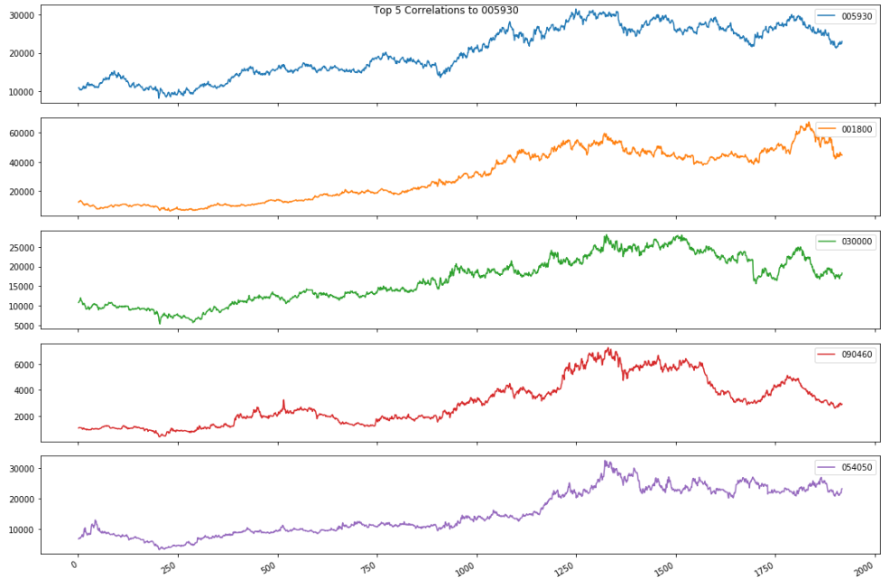
주가를 기반으로 유의미한 상관관계를 갖는 종목은 이와 같은 결과가 나왔습니다.

Input:

for key, value in top_correlated_companies.items():
    print('{} : {}'.format(company_list.loc[company_list.종목코드 == key, '회사명'].values[0], value))   

Output:

삼성전자 : 1.0
오리온홀딩스 : 0.9480981638541061
제일기획 : 0.9368736502664881
비에이치 : 0.9202494270558285
농우바이오 : 0.9143668553498088

위 목록에 대한 놀라운 사실은 오리온 홀딩스가 삼성그룹 계열사보다 삼성전자와 더 관련이 있다는 것입니다. 이것을 더 자세히 조사해 봅시다.

위와 같은 주식 차트처럼 "trendy"한 시계열 데이터에 대한 것 중 하나는 오해의 소지가 있는 결론으로 이어질 수 있습니다.

각 차트는 시간과 관련이 있기 때문에 한 주식 차트가 다른 차트에 대해 회귀 할 때 주가와 같은 "trendy"한 시계열 데이터가 까다로울 수 있습니다. 그들은 모두 시간과 상관 관계가 있기 때문에 강하지만, 종종 가짜 관계를 나타낼 것입니다.

따라서 주가와 같은 "trendy"한 시계열 데이터는 "nonstationary"로 간주됩니다.(즉, 시간에 따라 변화하는 평균 및 분산을 갖는 것)

그렇기 때문에 시계열 데이터를 처리 할 때 당신은 일반적으로 그들이 시간에 독립적으로 상관 관계가 있는지 알고 싶어할 것입니다. 한 series의 variations이 다른 것의 variations과 일치 하는지 여부를 알고 싶을 겁니다. 이 때, "Trend"의 존재는 당신을 혼동시킬 수 있으므로 피해야합니다.

따라서 데이터에서 "trend"을 제거하기 위해 다음의 작업을 수행했습니다.

먼저 전체 시계열을 1의 기간으로 차이를 두었습니다. 이것은 지난 기간동안 포트폴리오에서 모든 "일일 수익률"을 얻었음을 의미합니다. 우리는 이제 삼성전자의 일일 수익률과 가까운 correlation을 갖는 종목들로 비교할 것입니다.

우리의 데이터 프레임에 적용된 "diff (1)"함수로 pandas에서 이것을 쉽게 수행 할 수 있습니다. 우리는 기존의 주식 포트폴리오에서 differnce를 하도록 하겠습니다. .

Input:

all_df_diff = all_df.diff(1)
all_df_diff = all_df_diff.iloc[1:,:]
all_df_diff_T = all_df_diff.T
all_df_diff_T.reset_index(drop=False, inplace=True)

for col in incl:
    all_df_diff_T[col] = all_df_diff_T[col].map(lambda x: float(x))

top_correlated_companies = top_correlation_to_name(all_df_diff_T, 'index', '005930', 5, abs_corr=True)

for key, value in top_correlated_companies.items():
    print('{} : {}'.format(company_list.loc[company_list.종목코드 == key, '회사명'].values[0], value))   

Output:

삼성전자 : 1.0
삼성전기 : 0.4065839894458186
SK하이닉스 : 0.3751230260001406
LG디스플레이 : 0.36649793644842443
삼성증권 : 0.35648431858304086

새로운 차트의 흥미로운 점은 이전보다 삼성전자와의 상관관계가 훨씬 낮다는 것입니다. "trend"를 제거했음에도 불구하고 상관관계가 있는 종목들을 보면 기존의 결과와는 매우 다릅니다. 삼성의 계열사가 주를 이루고 관련되어 있는 종목들이 결과로 나오는 것을 확인할 수 있습니다. 이 간단한 tool을 통해서 우리는 상관관계가 있는 종목들을 도출해 낼 수 있습니다. 이처럼 시계열의 데이터에서 얻을 수 있는 "trend"가 있는 데이터는 분명히 차이를 둬야된다는 것은 매우 중요합니다.

다음 포스팅에서는 이 상관관계가 있는 종목 데이터를 이용하는 방법에 대해 알아보겠습니다.

Macroeconomic forecasting with Gaussian processes

정확한 거시경제 예측은 사업 결정, 금융 거래, 그리고 정치인과 경제학자들에 의한 정책 결정의 근거로서 필수적입니다. 전통적으로 시계열 데이터에 대한 선형 회귀 또는 밀접하게 관련된 방법을 통해 수행되었습니다. 

본 포스팅에서는 인기 있는 비선형적 방법인 가우스 프로세스 회귀 분석을 사용하여 여러 국가의 GDP를 예측하여 전통적인 기법보다 더 나은 결과를 얻을 수 있는지 여부를 확인하고자 합니다.

가장 중요한 거시경제변수는 아마도 국내총생산(GDP)일 것입니다. 그것은 한 지역에서 판매되는 모든 상품과 서비스의 가치를 측정하기 때문입니다. 따라서 우리는 GDP 예측에 초점을 맞출 것입니다.

전체적으로는 다음과 같이 구성됩니다.

1. 먼저 데이터를 로드하고 변환한 다음, 

2. simple baseline method 및 multivariate time-series regression을 평가하고 

3. 마지막으로 가우스 프로세스(GP) 회귀 분석과 비교합니다.

Environment

우리는 pandas, statsmodels, scikit-learn 패키지를 사용할 것입니다. 

콘솔이나 터미널에 아래와 같은 명령어로 설치합니다. 

    > pip3 install pandas
    > pip3 install statsmodels
    > pip3 install sklearn

Configuration

첫 째로, 우리는 configuration을 특정할 것입니다. 만약 다른 나라, 기간, indicators가 필요하다면 코드를 바꾸시면 됩니다.

Input:

# out-of-sample로 사용할 년도의 수 
#(실제 GDP와 비교하여 매년 국가별로 하나의 예측을 할 것입니다)
nyears = 10

# GP regression에 사용할 lag의 수
lags = 5

# Indicator labels과 the World Bank API에서의 이름
indicators  = {"gdp"        : "NY.GDP.MKTP.CD",
               "population" :    "SP.POP.TOTL",
               "inflation"  : "FP.CPI.TOTL.ZG"}
nindicators = len(indicators)

# 예측하기 위한 변수, indicator labels 중에 하나여야 함
target_variable = "gdp"

# Countries to include in the data, specified as ISO country codes
countries  = ['au','ca','de','es','fr','gb','jp','us']
ncountries = len(countries)

# 데이터 셋의 시작 연도와 마지막 연도
start_year = 1976
end_year   = 2018

Data

Loading

먼저 우리는 몇몇의 거시경제 지표들을 the World Bank HTTP API를 통하여 다운받을 것입니다. 여기서 Python의 requests 패키지를 사용하게 됩니다.

먼저 우리가 위에 configuration에서 설정했던 각각 다른 나라들, indicator로 채워질 template url을 특정합니다. 우리가 URL에 request할 때, 그 데이터들은 json 형식으로 fetched 될 것입니다. 우리는 그것들을 pandas dataframe에 넣을 것입니다.

import requests
import pandas as pd

template_url = "http://api.worldbank.org/v2/countries/{0}/indi"
template_url += "cators/{1}?date={2}:{3}&format=json&per_page=999"

# Countries는 세미 콜론으로 분리됩니다.
country_str = ';'.join(countries)
raw_data = pd.DataFrame()
for label, indicator in indicators.items():
    # template URL을 채웁니다.
    url = template_url.format(country_str, indicator, start_year, end_year)

    # 데이터를 request하고
    json_data = requests.get(url)

    # JSON String을 python object로 변경합니다.
    json_data = json_data.json()

    # 반환되는 데이터는 리스트이며, 첫 번째 element는 meta데이터,
    # 두 번째 element가 실제 데이터입니다.

    json_data = json_data[1]

    # 모든 데이터 포인트를 loop하며 value들을 dataframe으로 확장합니다.
    for data_point in json_data:
        country = data_point['country']['id']
        # 각각 나라, indicator로 variable을 만듬
        item = country + '_' + label

        year = data_point['date']

        value = data_point['value']

        # DataFrame으로 Append
        new_row = pd.DataFrame([[item, year, value]],
                               columns=['item', 'year', 'value'])
        raw_data = raw_data.append(new_row)
# 데이터를 피벗하여 columns을 따라 특정 연도를 얻고, rows를 따라 variable을 얻습니다.
raw_data = raw_data.pivot(index='year', columns='item', values='value')

# rows와 columns 출력 테스트
print('\n', raw_data.iloc[:10, :5], '\n')

Output:

Exploration

plots을 통해 데이터를 explore해보도록 하겠습니다.

Input:

import matplotlib.pyplot as plt

for lab in indicators.keys():
    
    indicator = raw_data[[x for x in raw_data.columns 
                              if x.split("_")[-1] == lab]]
    indicator.plot(title=lab)
    plt.show()

Output:

US의 GDP 성장율이 클수록 인구의 증가가 빠르다는 것을 부분적으로 설명할 수 있을 것입니다. 이것은 우리의 모델에 의해 captured 되어야 합니다.

Transformation

우리는 우리 모델의 데이터를 사용하기 전에, 적절한 모델로 transform해줘야 합니다.

Input:

import numpy as np

# 절대 값 대신에 우리는 상대적인 변화율을 이용할 것입니다.
# Nan값 때문에 오류가 발생할 수 있습니다.
data = np.log(raw_data).diff().iloc[1:,:]

# NaN을 0으로 채움.
data.fillna(0, inplace=True)

# 각 Series에서 평균값을 뺌
data = data - data.mean()

# index의 데이터 타입을 변경
data.index = pd.to_datetime(data.index, format='%Y')

# target variable 데이터만 뽑아서 target 변수에 넣음.
target = data[[x for x in data.columns if x.split("_")[-1] == target_variable]]

Evaluation

모든 모델들은 같은 방법으로 평가됩니다. 데이터의 마지막 연도를 예측하기 위해 우리는 각 나라의 이전 년도 데이터를 이용하여 모델을 훈련합니다. 각 예측에서 우리는 실제 값과 예측된 값의 차이를 제곱하여 error를 계산합니다. 그리고 mean을 구한 뒤, 제곱근을 취함으로써 우리는 root mean squared error (RMSE)를 구할 수 있습니다.

 ŷ𝒾 는 forecast 값,  𝘺𝒾 는 타겟 변수의 실제 값, 그리고 m은 우리가 예측할 년도의 개수입니다.

Baseline forecasts

우리는 먼저 simple baseline method 로 performance를 확인 해 본 뒤, subsequent methods와 비교해 볼 것입니다. baseline method는 간단하게 목표 변수의 이전 관측치와 동일한 변화율을 예측할 것입니다.

더 복잡한 방법은 naive baseline forecast보다 두드러지게 outperform하는 경우에만 사용하는 것이 좋습니다. the principle of Occam's Razor와 the KISS principle을 지키는 것이 좋습니다.

Input:

errors = target.iloc[-nyears:] - target.shift().iloc[-nyears:]

# Root mean squared error
rmse = errors.pow(2).sum().sum()/(nyears*ncountries)**.5

print('\n\t' + '-' * 18)
print("\t| Error: ", np.round(rmse, 4), '|')
print('\t' + '-' * 18 + '\n')

Output:

Multivariate time series

우리는 이제 multivariate time series regression의 performance를 조사해 볼 것입니다.

계량 경제학에서는 Vector Autoregression (VAR)이라고도 불립니다.

d는 독립 변수의 수, 𝜀는 lag의 수, εt 는 error term,  βi,jβi,j 는 추정된 파라미터입니다.

시계열 분석에 대한 자세한 내용을 알기 위해서는 Brockwell과 Davis의 "Time Series: Theory and Methods"와 Hamilton의 "Time Series Analysis"를 추천합니다.

모델을 fit하기 위해서 우리는 statsmodels 패키지를 사용합니다. 여기서 VAR 구현은 최소 제곱을 사용하여 매개 변수를 추정합니다. 하나의 lag를 이용하여 model을 훈련시킵니다. 즉, 독립 변수의 가장 최근 이전 값에서 대상 변수를 regression하지만, lag의 수를 설정을 지원하는 automatic methods도 있습니다. the Akaike Information Criterion (AIC) 나 Bayesian Information Criterion (BIC) 등이 있습니다.

Input:

from statsmodels.tsa.api import VAR

# Sum of squared errors
sse = 0

for t in range(nyears):
    
    # Create a VAR model
    model = VAR(target.iloc[t:-nyears+t], freq='AS')
    
    # Estimate the model parameters
    results = model.fit(maxlags=1)
    
    actual_values = target.values[-nyears+t+1]
    
    forecasts = results.forecast(target.values[:-nyears+t], 1)
    forecasts = forecasts[0,:ncountries]

sse += ((actual_values - forecasts)**2).sum()

# Root mean squared error
rmse = (sse / (nyears * ncountries))**.5

print('\n\t' + '-' * 18)
print("\t| Error: ", np.round(rmse, 4), '|')
print('\t' + '-' * 18 + '\n')

Output:

우리는 복잡한 VAR모델이 거시 경제 예측을 위해서 baseline model과 거의 동일하다는 것을 알 수 있습니다.

Gaussian process regression

우리는 이제 Gaussian process regression을 이용하여 GDP를 예측할 것입니다. 우리의 모델은 이전과 비슷합니다.

𝘺𝑡는 타겟 변수의 관측치입니다. 각 𝓍𝑡는 독립 변수의 관측된 벡터입니다.   𝑓(𝓍)는 regression 함수이고 noise term ε𝑡은 분산 α를 갖는 normal (Gaussian) distribution을 가지고 있습니다. 각 out-of-sample 예측에서 우리는 타겟 변수 y의 n년 간의 관측된 값을 column vector로 넣고 y로 나타낼 것입니다. 우리는 또한 각 관측치가 행렬에서 행을 차지하는 n년간 독립 변수의 관측치의 matrix를 X라고 할 것입니다. 여기서 각 관찰은 변수의 lagged values들을 포함할 것입니다.

회귀 함수 𝑓 (𝓍)가 임의의 매개 변수를 가진 선형 함수인 대신에, 함수는 이제 랜덤한 값을 가지므로 각 점 𝓍𝑡에서의 값은 정규 분포의 확률 변수이고 두 개의 확률 변수 𝑓(𝓍𝑡)와 𝑓(𝓍𝑠)는 소위 공분산 함수 (또는 커널) 𝑘(𝓍𝑡, 𝓍𝑠)에 의해 주어지며, 이것들은 지정되어야 합니다. 𝑓(𝓍) 함수는 '가우시안 프로세스'라 불립니다. error term이 정상적으로 분포되기 때문에 목표 값은 𝑡 = s이고 𝑘 (𝓍𝑡, 𝓍𝑠) 이면 𝑘 (𝓍𝑡, 𝓍𝑠) +𝑎 와 같은 공분산으로 정규 분포됩니다.

𝘺𝑡 와𝓍𝑡 에 대해 nn 개의 데이터 포인트를 사용하여 모델을 추정하고, 우리가 ŷ 𝑛+₁ 의 예측을 토대로 새로운 테스트 포인트 𝓍𝑛+₁을 가지고 있다고 가정합시다. 주어진 y, 𝑋 ,𝓍𝑛+₁ 에서 f(𝓍𝑛+₁) 의 조건부 분포는 또한 정규 분포를 가지며  ŷ𝑛+₁ 의 예측을 𝑓(𝓍𝑛+₁)의 조건부 기대 값으로 삼을 수 있습니다.  잘 알려진 공식인 multivariate Gaussian distribution은 아래와 같습니다.

K는 n X n 행렬 (행 t와 열 s에 대한 엔트리는  𝑘 (𝓍𝑠, 𝓍𝑡)로 주어지고, 𝐼는 항등 행렬이며, 𝐤는 𝑘(𝓍𝑡,𝓍𝑛+₁)에 의해 주어진 t를 갖는 길이 n의 열 벡터입니다.

classification에도 사용되는 Gaussian process methods를 더 읽기 위해서는, Rasmussen 과 Williams의 "Gaussian Processes in Machine Learning"을 보는 것을 추천합니다.

Gaussian process regression은 scikit-learn 패키지를 이용합니다. 각 예측 연도에 대해 과거 타겟 변수의 관측치들의 벡터 y와 독립 변수의 관측치들의 data matrix X를 생성합니다.

우리는 이것들을 GaussianProcessRegressor 클래스에 제공하여 모델을 estimate한 다음 다음 해에 대한 예측을 할 것입니다. 이전과 마찬가지로 RMSE를 사용하여 오류를 계산합니다.

우리는 아래와 같은 common Gaussian covariance function을 사용할 것입니다.

∥v∥ 는  vector vv의 길이이고 , σσ 는 매개변수입니다.

Input:

from sklearn.gaussian_process import GaussianProcessRegressor
from sklearn.gaussian_process.kernels import RBF

# 우리는 covariance function의 매개변수를 일반적인 covariance function의
# heuristic인 데이터 포인트의 median으로 사용합니다.
# The 'alpha' 인수는 잡음 분산이며, 우리가 covariance 매개변수와 동일하게 설정합니다.

gpr = GaussianProcessRegressor(kernel=RBF(0.1), alpha=0.1)
# 각 예측의 estimation/fitting을 위한 데이터 포인트의 수
ndata = target.shape[0] - nyears - lags
print(ndata)
# Sum of squared errors
sse = 0
for t in range(nyears):

    # 타겟 변수의 관측치
    y = np.zeros((ndata, ncountries))
    # 독립 변수의 관측치
    X = np.zeros((ndata, lags * ncountries * nindicators))

    for i in range(ndata):
        y[i] = target.iloc[t + i + 1]
        X[i] = data.iloc[t + i + 2:t + i + 2 + lags].values.flatten()

    gpr.fit(X, y)

    x_test = np.expand_dims(data.iloc[t + 1:t + 1 + lags].values.flatten(), 0)
    forecast = gpr.predict(x_test)

    sse += ((target.iloc[t].values - forecast) ** 2).sum()

rmse = (sse / (nyears * ncountries)) ** .5
print('\n\t' + '-' * 18)
print("\t| Error: ", np.round(rmse, 4), '|')
print('\t' + '-' * 18 + '\n')

Output:

우리는 지금까지 얻은 결과를 정리해보면 Gaussian process regression을 사용하여 얻은 결과는 baseline과 linear regression models과 비교하여 약간의 성능 개선이 있다는 것을 확인할 수 있었습니다.

옵션 가격결정 & The "Greeks"

1. 옵션 가격결정

이번 포스팅은 옵션 가격 결정과 Greeks에 대해 알아보도록 하겠습니다.

the Greeks를 이해하는 것, 내재 변동성, time decay(감쇠) 등 옵션 가격에 영향을 주는 요소들을 고려해 주는 것은 이 산업에서 성공적인 비지니스를 이룰 수 있는지와 없는지를 구별해 줄만큼 매우 중요한 요소입니다.

하지만 시장 변화에 따라 단일 옵션 또는 복수의 옵션이 포함된 포지션의 가격에 어떤 일이 발생할지 예측하는 것은 어려울 수 있습니다. 옵션은 많은 다른 요소들이 포함되어 있기 때문입니다. 따라서 옵션가격이 항상 주식의 가격과 함께 움직이는 것처럼 보이지 않기 때문에, 어떤 요소들이 옵션의 가격에 기여하고 그들이 가지는 영향을 이해하는 것이 중요합니다.

옵션 트레이더들은 종종 옵션 포지션의 델타, 감마, 베가, 세타를 이용합니다. 이것들은 종합적으로 "Greeks"라고 불리며 수량화 할 수있는 팩터들에 대한 옵션 가격의 민감도를 측정할 수 있는 방법입니다.

여기서 사람들이 흔히들 착각을 합니다. 중요한 것은, Greeks는 가격을 결정하는 것이 아니라는 것입니다. Greeks는 단지 주가 변동, 내재 변동성, 시간 등에 대한 옵션가격 변동이 일어날 수 있는 것을 반영합니다. 즉, Greeks는 앞을 내다보는 용도이지, 가격 결정을 하는 것이 아니라는 것입니다. 이것은 아주 중요한 차이입니다.

 
옵션 가격은 크게는 두 개의 카테고리로 분류가 됩니다.
첫 번째는 Intrinsic Value(내재 가치), Time Value(시간 가치)입니다.


1.1. Intrinsic Value


내재 가치에 대해 먼저 알아보자면,
만약 당신이 50의 Strike Price(행사가격)를 가지고 있는 콜 옵션이 있고
현재 Spot Price(현물가격)가 55라면 당신은 옵션의 5의 내재 가치를 가지고 있는 것입니다.
왜냐하면 당신은 50에 산 뒤, 즉시 55에 팔 수 있기 때문이죠.
간단하게 행사가격과 현물가격의 차이라고 생각할 수 있습니다.


1.2. Time Value

두 번째로는 시간 가치입니다.
이것이 문제입니다. 사람들은 대부분 내재 가치는 쉽게 얻지만, 이 시간 가치가 기초 자산의 가격 변동과 더불어 옵션 가격 변동에 많은 관련이 있기 때문입니다.
내재 가치는 linear한 관계에 있다면 이 시간 가치는 약간 다릅니다.


1.2.1. Time to Maturity


먼저 Time to Maturity(기간)은 만기가 얼마나 남았는지 입니다.
만기가 긴 옵션은 더 고평가 됩니다. 왜냐하면 그 계약이 성사되기 까지 시간이 오래 걸리기 때문입니다.


1.2.2. Volatility


다음은 Volatility(변동성)입니다. 이것은 여기서 핵심 요소입니다.
변동성이 높다면 옵션 가격은 상승합니다. 콜, 풋 모든 쪽에서 상승하게 되는데, 기초자산의 변동성이 크면 클수록 기초자산의 가격이 행사가격을 넘어 In-the-Money상태로 갈 확률이 높아지게 됩니다. 하루에 0.1%씩 오르고 내리는 주식 보다는 상한가 하한가를 보이며 움직이는 주식이 더 높은 옵션프리미엄을 가진다는 이야기입니다.


1.2.3. Rate of Interest


마지막으로는 Rate of Interest(이자율)입니다.
이것은 rho입니다. 여기서는 rho에 대해서 자세하게 설명하지 않겠습니다. 이것은 Time to Maturity와 Volatility 같이 계약 만기가 더 길어질수록 이자율은 옵션 가치에 더 큰 영향을 미치게 됩니다. 60일 이내의 옵션의 경우에는 이것의 영향이 거의 존재하지 않습니다.
그렇기 때문에 main Greek으로 다루진 않겠지만 이러한 것이 있다는 것을 알아두면 좋게습니다.

이렇게 기본적인 옵션 가격결정에 대해 알아보았으며, 이제는 실제 Greek에 대해 알아 보도록 하겠습니다.

2. The Greeks

우리가 좀 전까지 다뤘던 Option Pricing을 Greeks으로 바꿔보면 그림과 같이 5가지의 Greeks이 있습니다. 기본적으로 4가지의 중요한 Greeks은 Delta, Gamma, Vega, Theta입니다. 그리고 Rho까지 총 5가지의 Greeks입니다. 여기서 Rho는 중요 요소가 아니지만 무시하지는 않을 것입니다.

2.1. Delta

델타(Delta) = 옵션가격변화 / 기초자산의 변화

델타는 기본적으로 내재 가치에 대한 관계를 보여주는 역할을 합니다. 기초 자산의 변화에 따른 옵션 가치의 변화로 표현합니다.

만약 콜옵션이 Deep OTM(깊은 외가격상태)에 있을 경우 콜옵션의 델타는 0에 가까울 것입니다. 만약 기초자산의 가격이 조금 오르더라도 콜옵션은 아직 OTM일 것이기 때문에 가격의 변화가 거의 없을 것이기 때문입니다.

그리고 콜옵션이 Deep ITM에 있는 경우 콜옵션의 델타는 거의 1에 가까울 것입니다.

기초 자산 가격변화와 거의 같은 비율로 콜옵션의 가격이 변하게 될 것이기 때문입니다.

2.2. Gamma

감마(Gamma) = 델타 가격변화 / 기초자산의 변화

감마는 맨 위 그림과 연결되진 않지만 델타와 관련이 있습니다. 감마는 기본적으로 변화율, 혹은 델타의 acceleration amount입니다.

2.3. Vega

Vega-Volatility. 

베가(Vega) = 옵션 가격변화 / 주가지수의 변화

외우기 쉽죠. 베가는 기초자산의 가격변동성의 변화에 따른 옵션가격의 변화 정도를 말합니다.

가격 변동성은 말씀 드렸다시피 시간가치를 결정하는 데에 가장 중요한 변수입니다. 변동성이 증가하면 시장의 불확실성이 높아져 시간가치가 증가하죠.

가격 변동성이 상승할 것을 예상한다면 등가격 옵션의 매수를 고려하고, 반대일 경우에는 매도를 고려합니다. 이는 등가격옵션의 베가가 가장 크기 때문입니다.

2.4. Theta

Theta-Time to Maturity.

세타(Theta) = 옵션 가격변화 / 시간의 변화

세타는 시간의 경과함에 따른 옵션가격의 변화 정도를 말합니다. 옵션은 만기일에 가까워질수록 시간가치가 줄어듭니다. 세타는 이러한 시간소멸효과를 측정한 것으로, 현재의 옵션시장가격과 익일의 이론가격과의 차이를 나타냅니다.

세타는 베가와 마찬가지로 등가격옵션일 때 가장 크고 내가격이나 외가격으로 갈수록 작아지게 됩니다.

2.5. Rho

Rho - Rate of Interest

로(Rho) = 옵션 가격변화 / 이자율의 변화

로는 이자율의 변화에 따른 옵션값의 변화를 뜻합니다. 일반적으로 콜옵션 매수자는 금리가 오르면 유리하고 반대로, 풋옵션 매수자는 금리가 내려가면 유리합니다.

피오트로스키의 F-score를 이용하여 미국 시장에 백테스팅 해 볼 예정입니다.

피오트로스키는 재무제표에 대한 점수를 아래와 같이 나눕니다.

1. 수익성2. 재무건전성3. 효율성

How the Piotroski F-Score Stock Screen Works

The F-Score Test examines 9 tests in three areas: profitability, capital structure, and operating efficiency. Each test is given either 0 points for a fail or 1 point for a pass. All 9 tests can be derived from company financial statements.

Piotroski found that companies with 8 or 9 total points greatly improved the probability that the company had the ability to overcome challenges and eventually grow its stock price. Here are the 9 tests in the 3 areas:

Profitability (4 points)

Return on Assets

Return on assets (ROA) is net income before extraordinary items divided by total assets. If ROA is positive award 1 point; if negative, no points.

Cash Flow from Operations

Cash Flow From Operations is the cash inflows and outflows of a company’s core business operations. One point is awarded for positive cash flow from operations and none if it is negative.

Direction of Return on Assets

Did the return on assets increase this year over last year? Is so, award 1 point; if not, no points.

Accrual Accounting Check

Does the cash from operations exceed net income before extraordinary items? If yes, award 1 point, if not, no points.

Capital Structure (3 points)

Direction of Leverage

Did the long term debt to total assets ratio increase or decrease from the year before? If leverage decreased award 1 point; if it increased, no points.

Direction of Liquidity

Did the current ratio (current assets divided by current liabilities) increase or decrease from the prior year? If it increased, award 1 point; if it decreased, no points.

Issue Stock

When a company issues stock it dilutes the present shareholders stake and may indicate the company is unable to raise sufficient capital from operations. If the company has not issued stock in the past year award 1 point; if it issued stock, 0 points.

Operating Efficiency (2 points)

Direction of Margin

If the gross margin ratio has increased (year over year) that is a positive sign, award 1 point. Falling margins would be a warning sign, no points awarded.

Direction of Asset Turnover

An increase in asset turnover (sales divided by assets at the beginning of the year) from one year to another would indicate greater efficiency. Award 1 point for a higher asset turnover ratio than the previous year; 0 points if it has decreased.

1.a. max_features:

만들어지는 나무의 갯수 :

1. Auto/None : This will simply take all the features which make sense in every tree.Here we simply do not put any restrictions on the individual tree.
2. sqrt : This option will take square root of the total number of features in individual run. For instance, if the total number of variables are 100, we can only take 10 of them in individual tree.”log2″ is another similar type of option for max_features.
3. 0.2 : This option allows the random forest to take 20% of variables in individual run. We can assign and value in a format “0.x” where we want x% of features to be considered.

How does “max_features” impact performance and speed?

Increasing max_features generally improves the performance of the model as at each node now we have a higher number of options to be considered. However, this is not necessarily true as this decreases the diversity of individual tree which is the USP of random forest. But, for sure, you decrease the speed of algorithm by increasing the max_features. Hence, you need to strike the right balance and choose the optimal max_features.

1.b. n_estimators :

This is the number of trees you want to build before taking the maximum voting or averages of predictions. Higher number of trees give you better performance but makes your code slower. You should choose as high value as your processor can handle because this makes your predictions stronger and more stable.

1.c. min_sample_leaf :

If you have built a decision tree before, you can appreciate the importance of minimum sample leaf size. Leaf is the end node of a decision tree. A smaller leaf makes the model more prone to capturing noise in train data. Generally I prefer a minimum leaf size of more than 50. However, you should try multiple leaf sizes to find the most optimum for your use case.

2. Features which will make the model training easier

There are a few attributes which have a direct impact on model training speed. Following are the key parameters which you can tune for model speed :

2.a. n_jobs :

This parameter tells the engine how many processors is it allowed to use. A value of “-1” means there is no restriction whereas a value of “1” means it can only use one processor. Here is a simple experiment you can do with Python to check this metric :

%timeit

model = RandomForestRegressor(n_estimator = 100, oob_score = TRUE,n_jobs = 1,random_state =1)

model.fit(X,y)

Output  ———-  1 loop best of 3 : 1.7 sec per loop

%timeit

model = RandomForestRegressor(n_estimator = 100,oob_score = TRUE,n_jobs = -1,random_state =1)

model.fit(X,y)

Output  ———-  1 loop best of 3 : 1.1 sec per loop

“%timeit” is an awsum function which runs a function multiple times and gives the fastest loop run time. This comes out very handy while scalling up a particular function from prototype to final dataset.

2.b. random_state :

This parameter makes a solution easy to replicate. A definite value of random_state will always produce same results if given with same parameters and training data. I have personally found an ensemble with multiple models of different random states and all optimum parameters sometime performs better than individual random state.

2.c. oob_score :

This is a random forest cross validation method. It is very similar to leave one out validation technique, however, this is so much faster. This method simply tags every observation used in different tress. And then it finds out a maximum vote score for every observation based on only trees which did not use this particular observation to train itself.

Here is a single example of using all these parameters in a single function :

model = RandomForestRegressor(n_estimator = 100, oob_score = TRUE, n_jobs = -1,random_state =50,                                         max_features = "auto", min_samples_leaf = 50)

model.fit(X,y)

Learning through a case study

We have referred to Titanic case study in many of our previous articles. Let’s try the same problem again. The objective of this case here will be to get a feel of random forest parameter tuning and not getting the right features. Try following code to build a basic model :

from sklearn.ensemble import RandomForestRegressor

from sklearn.metrics import roc_auc_score

import pandas as pd

x = pd.read_csv("train.csv")

y = x.pop("Survived")

model =  RandomForestRegressor(n_estimator = 100 , oob_score = TRUE, random_state = 42)

model.fit(x(numeric_variable,y)

print "AUC - ROC : ", roc_auc_score(y,model.oob_prediction)

AUC – ROC : 0.7386

This is a very simplistic model with no parameter tuning. Now let’s do some parameter tuning. As we have discussed before, we have 6 key parameters to tune. We have some grid search algorithm built in Python, which can tune all parameters automatically.But here let’s get our hands dirty to understand the mechanism better. Following code will help you tune the model for different leaf size.

Exercise : Try runing the following code and find the optimal leaf size in the comment box.

sample_leaf_options = [1,5,10,50,100,200,500]

for leaf_size in sample_leaf_options :

     model = RandomForestRegressor(n_estimator = 200, oob_score = TRUE, n_jobs = -1,random_state =50,                                         max_features = "auto", min_samples_leaf = leaf_size)

     model.fit(x(numeric_variable,y)

     print "AUC - ROC : ", roc_auc_score(y,model.oob_prediction)

HFT에 필요한 네트워크인 TOE와 RDMA에 관한 분석입니다.
발표자료를 만들어보았습니다.
I made this one for presentation.
This is about TOE, RDMA for HFT.