Correlated assets
2) 역사는 반복된다.
3) 시장은 사람들의 합리적인 행동에 따른다.
4) 시장은 'perfect'하다.
우리는 이러한 가정을 한 뒤, 삼성전자(005930) 의 주가 움직임을 예측해 볼 것입니다.
우리는 삼성전자의 주가가 등락 여부에 어떤 것들이 영향을 주는 지를 이해해야 합니다. 그러므로, 우리는 가능한 많은 정보를 통합할 것입니다. (주식을 다양한 방면과 각도로 묘사하기 위해) 우리는 일별 데이터 (우리가 가지고 있는 데이터의 70%) 를 사용하여 다양한 알고리즘을 훈련시키고 나머지를 예측하는데 사용할 것입니다. 그리고 우리는 예측된 결과와 hold-out 데이터를 비교할 것입니다. .
이것들은 꼭 주식이 아니더라도 원자재, FX, 지수, 채권 등 아무 유형이 가능합니다.
삼성전자와 같은 큰 기업은 고립되어 있지 않습니다. 경쟁사를 포함하여 고객들, 글로벌 경제, 지정학적 현상, 재정 및 통화 정책, 자본 접근 등 외부요인이 있습니다.
Correlated stocks
이번 포스팅에서는 먼저 삼성전자와 유의미한 상관관계를 갖고 있는 기업들을 찾아볼 것입니다. 전체적으로는 상관관계가 있는 기업을 찾기 위해, 종가데이터를 이용하여 correlation을 구하는 것 방법의 문제점과 해결 방법에 대해 알아보도록 하겠습니다.
Environment
import pandas as pd
import numpy as np
from sklearn.model_selection import train_test_split
Configuration
Input:
2008년 1월 2일부터 2019년 1월 25일의 데이터를 사용할 것입니다. (7년은 training 목적, 3년은 validation 목적)
Input:
train, test = train_test_split(samsung_df, test_size=0.3, shuffle=False)
print('There are {} number of days in the dataset.'.format(samsung_df.shape[0]))
print('train set : {}, test set : {}'.format(train.shape[0], test.shape[0]))
print('train period : {} ~ {}'.format(train.index[0], train.index[-1]))
print('test period : {} ~ {}'.format(test.index[0], test.index[-1]))
Output:
There are 2739 number of days in the dataset.
train set : 1917, test set : 822
train period : 2008-01-02 ~ 2015-09-16
test period : 2015-09-17 ~ 2019-01-25

먼저 전체 주가 데이터를 symbol을 column으로 하여 데이터프레임을 생성한 뒤 데이터를 입력합니다.
Input:
all_df.head(2)
Output:

이제 특정 기업과 나머지 모든 기업에 대한 correlation을 구합니다. 여기서 먼저 correlation을 구하기 위한 함수를 정의해줍니다. 종목들마다 종가데이터가 있는 정도가 다르기 때문에 nan값에 대한 처리를 해주는 것이 중요합니다.
def search_string(gr, column, strings_list):
    if isinstance(strings_list,str):
        strings_list = [strings_list]
    if isinstance(column, str):
        #### if column is not a list but a string, it means there is only one column to search
        return gr[gr[column].str.contains('|'.join(strings_list),na=False)]
    else:
        gr_df = pd.DataFrame()
        counter = 0
        for col in column:
            if counter == 0:
                gr_df =  gr[gr[col].str.contains('|'.join(strings_list),na=False)]
                counter += 1
            else:
                gr_df.append(gr[gr[col].str.contains('|'.join(strings_list),na=False)])
                counter += 1
        return gr_df


def top_correlation_to_name(stocks, column_name, searchstring, top=10, abs_corr=False):
    incl = [x for x in list(stocks) if x not in column_name]
    ### First drop all NA rows since they will mess up your correlations.
    stocks.dropna(inplace=True)
    ### Now find the highest correlated rows to the selected row ###
    try:
        index_val = search_string(stocks, column_name,searchstring).index[0]
    except:
        print('Not able to find the search string in the column.')
        return
    ### Bring that selected Row to the top of the Data Frame
    df = stocks[:]
    df["new"] = range(1, len(df)+1)
    df.loc[index_val,"new"] = 0
    stocks = df.sort_values("new").drop("new",axis=1)
    stocks.reset_index(inplace=True,drop=True)
    ##### Now calculate the correlation coefficients of other rows with the Top row
    try:
        if abs_corr == True:
            cordf = pd.DataFrame(stocks[incl].T.corr().abs().sort_values(0,ascending=False))
        else:
            cordf = pd.DataFrame(stocks[incl].T.corr().sort_values(0,ascending=False))
    except:
        print('Cannot calculate Correlations since Dataframe contains string values or objects.')
        return
    try:
        cordf = stocks[column_name].join(cordf)
    except:
        cordf = pd.concat((stocks[column_name],cordf),axis=1)
    #### Visualizing the top 5 or 10 or whatever cut-off they have given for Corr Coeff
    if top >= 1:
        top10index = cordf.sort_values(0,ascending=False).iloc[:top,:3].index
        top10names = cordf.sort_values(0,ascending=False).iloc[:top,:3][column_name]
        top10values = cordf.sort_values(0,ascending=False)[0].values[:top]
    else:
        top10index = cordf.sort_values(0,ascending=False)[
            cordf.sort_values(0,ascending=False)[0].values>=top].index
        top10names = cordf.sort_values(0,ascending=False)[
            cordf.sort_values(0,ascending=False)[0].values>=top][column_name]
        top10values = cordf.sort_values(0,ascending=False)[
            cordf.sort_values(0,ascending=False)[0].values>=top][0]
    #### Now plot the top rows that are highly correlated based on condition above
    stocksloc = stocks.iloc[top10index]
    #### Visualizing using Matplotlib ###
    stocksloc = stocksloc.T
    stocksloc = stocksloc.reset_index(drop=True)
    stocksloc.columns = stocksloc.iloc[0].values.tolist()
    stocksloc.drop(0).plot(subplots=True, figsize=(15,10),legend=False,
                         title="Top %s Correlations to %s" %(top,searchstring))
    [ax.legend(loc=1) for ax in plt.gcf().axes]
    plt.tight_layout()
    plt.show()

    return dict(zip(top10names, top10values))
그 후, 함수를 사용하기 위해 전처리를 해줍니다.
Input:
all_df_T = all_df.T
all_df_T.reset_index(drop=False, inplace=True)
all_df_T.head(1)

for col in incl:
    all_df_T[col] = all_df_T[col].map(lambda x: float(x))
Output:

Input:
top_correlated_companies = top_correlation_to_name(all_df_T, 'index', '005930', 5, abs_corr=True)
Output:
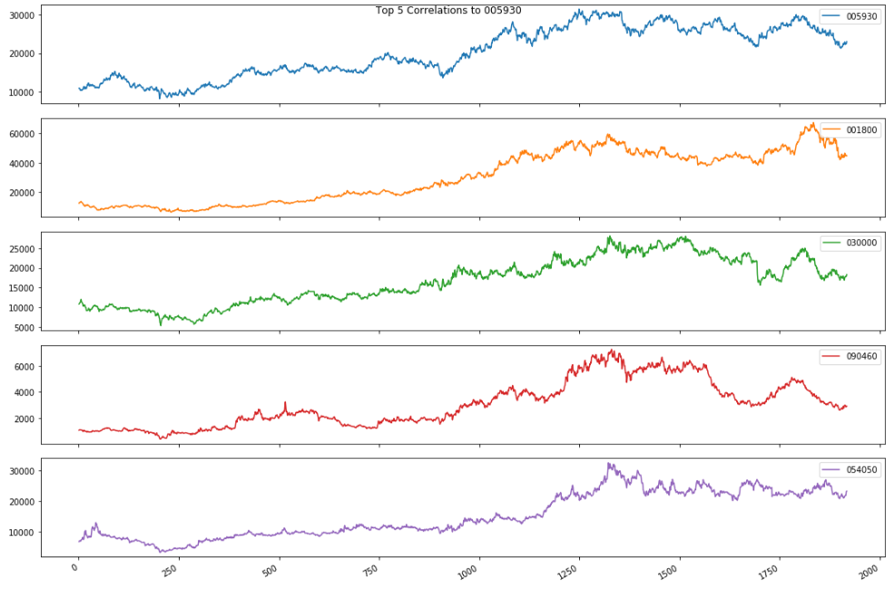
주가를 기반으로 유의미한 상관관계를 갖는 종목은 이와 같은 결과가 나왔습니다.
Input:
for key, value in top_correlated_companies.items():
    print('{} : {}'.format(company_list.loc[company_list.종목코드 == key, '회사명'].values[0], value))
Output:
삼성전자 : 1.0
오리온홀딩스 : 0.9480981638541061
제일기획 : 0.9368736502664881
비에이치 : 0.9202494270558285
농우바이오 : 0.9143668553498088
위 목록에 대한 놀라운 사실은 오리온 홀딩스가 삼성그룹 계열사보다 삼성전자와 더 관련이 있다는 것입니다. 이것을 더 자세히 조사해 봅시다.
위와 같은 주식 차트처럼 "trendy"한 시계열 데이터에 대한 것 중 하나는 오해의 소지가 있는 결론으로 이어질 수 있습니다.
각 차트는 시간과 관련이 있기 때문에 한 주식 차트가 다른 차트에 대해 회귀 할 때 주가와 같은 "trendy"한 시계열 데이터가 까다로울 수 있습니다. 그들은 모두 시간과 상관 관계가 있기 때문에 강하지만, 종종 가짜 관계를 나타낼 것입니다.
따라서 주가와 같은 "trendy"한 시계열 데이터는 "nonstationary"로 간주됩니다.(즉, 시간에 따라 변화하는 평균 및 분산을 갖는 것)
그렇기 때문에 시계열 데이터를 처리 할 때 당신은 일반적으로 그들이 시간에 독립적으로 상관 관계가 있는지 알고 싶어할 것입니다. 한 series의 variations이 다른 것의 variations과 일치 하는지 여부를 알고 싶을 겁니다. 이 때, "Trend"의 존재는 당신을 혼동시킬 수 있으므로 피해야합니다.
따라서 데이터에서 "trend"을 제거하기 위해 다음의 작업을 수행했습니다.
먼저 전체 시계열을 1의 기간으로 차이를 두었습니다. 이것은 지난 기간동안 포트폴리오에서 모든 "일일 수익률"을 얻었음을 의미합니다. 우리는 이제 삼성전자의 일일 수익률과 가까운 correlation을 갖는 종목들로 비교할 것입니다.
우리의 데이터 프레임에 적용된 "diff (1)"함수로 pandas에서 이것을 쉽게 수행 할 수 있습니다. 우리는 기존의 주식 포트폴리오에서 differnce를 하도록 하겠습니다. .
Input:
all_df_diff = all_df.diff(1)
all_df_diff = all_df_diff.iloc[1:,:]
all_df_diff_T = all_df_diff.T
all_df_diff_T.reset_index(drop=False, inplace=True)

for col in incl:
    all_df_diff_T[col] = all_df_diff_T[col].map(lambda x: float(x))

top_correlated_companies = top_correlation_to_name(all_df_diff_T, 'index', '005930', 5, abs_corr=True)

for key, value in top_correlated_companies.items():
    print('{} : {}'.format(company_list.loc[company_list.종목코드 == key, '회사명'].values[0], value))
Output:

삼성전자 : 1.0
삼성전기 : 0.4065839894458186
SK하이닉스 : 0.3751230260001406
LG디스플레이 : 0.36649793644842443
삼성증권 : 0.35648431858304086
새로운 차트의 흥미로운 점은 이전보다 삼성전자와의 상관관계가 훨씬 낮다는 것입니다. "trend"를 제거했음에도 불구하고 상관관계가 있는 종목들을 보면 기존의 결과와는 매우 다릅니다. 삼성의 계열사가 주를 이루고 관련되어 있는 종목들이 결과로 나오는 것을 확인할 수 있습니다. 이 간단한 tool을 통해서 우리는 상관관계가 있는 종목들을 도출해 낼 수 있습니다. 이처럼 시계열의 데이터에서 얻을 수 있는 "trend"가 있는 데이터는 분명히 차이를 둬야된다는 것은 매우 중요합니다.
다음 포스팅에서는 이 상관관계가 있는 종목 데이터를 이용하는 방법에 대해 알아보겠습니다.


0 개의 댓글:
댓글 쓰기